Vorbereitung - Programmiertools

`R`

Benötigte `R`-Pakete installieren

Auswahl folgender Pakete sollte für die Bearbeitung der Aufgaben und das Nachimplementieren der Anwendungen aus den Studienbriefen ausreichend sein:

#| cache: true
install.packages(
  c("rcompanion", "polr", "ordinal", "DescTools", "tidyverse", "ggplot2", "dplyr",
    "PerformanceAnalytics", "rugarch", "tsibbledata", "mFilter", "FinTS",
    "plm")
)

Rest der Veranstaltung: R-code – daher eine kleine Wiederholung zu Python weiter unten.

########################### Allgemeine Grundlagen #####
test      <- 5             # Kommentarbereich
testplus  <- test + 5      # Addition
testminus <- testplus - 3  # Subtraktion
testdiv   <- testminus / 7 # Division
testmult  <- testdiv * 4   # Multiplikation

v <- c(1, 2, 10, 5, 6, 7) # Vektor
v[3]
v[1:4]
v[v < 3]
l <- list(v = c(1,2), f = c("a", "b"))
l$v
l[1:2]
l[[2]]
l["v"]


mymatrix <- matrix(data = c(1,2,3,4,5,6), nrow = 2, ncol = 3)
mymatrix[1,2]
mymatrix[, 3]
mymatrix[2, ]

mydf <- data.frame(name1 = c(1,2),name2 = c(3,4), name3 = c(5,6))
mydf[1,2]
mydf$name3[1]
mydf[,3]
mydf$name1
mydf[2, ]

########################### Pakete installieren #####
#install.packages("tidyverse")
library(tidyverse)
########################### Daten einlesen #####
mydata <- readxl::read_xls("bsp_file.xlsx")
mydata <- read.csv("bsp_file.csv")
mydata <- foreign::read.dta("bsp_file.dta")
testme <- load("bsp_file.rda")

########################### Conditional Code #####
for (i in c(1, 3, 5)) {
  print(i)
}
while (i <= 4) {
print("i is still smaller or equal to 4")
}


if (i <= 4) {
  print(i)
} else {
  print("i is not smaller 4")
}

# Logische Operationen
a <- 3
b <- 4

a == b
a != b
a > b
a >= b
a <- NA
b <- "text ist hier"
is.na(a)
!is.na(b)

########################### Funktionen definieren #####
bsp_funktion <- function(x, y) {
 muffin <- c(x + y, x * y, x - y)
 return(muffin)
}


########################### Datenmanipulation #####
head(mtcars)
library(magrittr) # fuer den Pipe-operator
mtcars %>%
  dplyr::select(mpg, hp)

library(dplyr)
mtcars %>%
  select(mpg, hp)

mtcars %>% head() %>% filter(cyl %in% 4:6)
#



########################### ggplot 2 Intro #####
library(ggplot2)
ggplot(data = iris,
aes(x = Petal.Length,
y = Sepal.Length)) +
geom_point()

ggplot(data = iris,
aes(x = Petal.Length,
y = Sepal.Length,
color = Species)) +
geom_point()

ggplot(data = iris,
aes(x = Petal.Length,
y = Sepal.Length,
shape = Species)) +
geom_point()

ggplot(data = iris,
aes(x = Petal.Length,
y = Sepal.Length,
color = Species,
shape = Species)) +
geom_point()

ggplot(data = wb_data[which(
wb_data$`Country Name` == 'Haiti'), ],
aes(x = variable, y = value)) +
geom_line() +
ylim(25, 50) +
xlim(1995, 2020)

ggplot(data = wb_data[which(
wb_data$`Country Name` == 'Haiti' |
wb_data$`Country Name` == 'India'), ],
aes(x = variable,
y = value,
color = `Country Name`)) +
geom_line() +
ylim(25, 100) +
xlim(1995, 2020) +
theme(legend.position = 'bottom')

ggplot(data = wb_data,
aes(x = `Country Name`)) +
geom_bar(stat = 'count') +
coord_flip()

ggplot(data = wb_mean,
aes(x = Mean, y = Country)) +
geom_bar(stat = 'identity') +
geom_errorbar(aes(xmin = Mean - SD,
xmax = Mean + SD), width = 0.6,
alpha = 0.9, size = 1,
color ='red', stat = "identity")


ggplot(data = wb_mean,
aes(x = Mean,
y = reorder(Country, -Mean))) +
geom_bar(stat = 'identity') +
geom_errorbar(aes(xmin = Mean - SD,
xmax = Mean + SD), width = 0.6,
alpha = 0.9, size = 1,
color='red', stat = "identity")


ggplot(data = iris, aes(
x = Petal.Length,
y = Sepal.Length)) +
geom_point() +
facet_wrap(vars(Species))

ggplot(data = iris, aes(
x = Petal.Length,
y = Sepal.Length)) +
geom_point() +
facet_wrap(vars(Species),
nrow = 3)



# install.packages("ggpubr")
library(ggpubr)

scatter_1 <- ggplot(data = iris, aes(x = Petal.Length,
y = Sepal.Length)) +
geom_point()

line_2 <- ggplot(data = wb_data[which(
wb_data$`Country Name` == 'Haiti' |
wb_data$`Country Name` == 'India'), ],
aes(x = variable,
y = value,
color = `Country Name`)) +
geom_line() +
ylim(25, 100) +
xlim(1995, 2020) +
theme(legend.position = 'bottom')


ggarrange(scatter_1, line_2,
labels = c('Erster Scatterplot',
'Zweites Liniendiagram'),
legend = 'bottom')

Python

Grundlagen
Ein Python Tupel: geordnet aber nicht veränderbar
```
mytuple = ("apple", "banana", "cherry")
```

Python Liste: geordnet und veränderbar

test = 5*5
a_bool = True
b_bool = False
# comment; like R
"""
this is a longer comment
"""
mylist_01 = [1, "FSM", 3, True]       # direkte Konstruktion
mylist_02 = list((1, "FSM", 3, True)) # Konstruktion über Tupel (iterable)
# INDEXING STARTET BEI NULL vs. R BEI 1
mylist_01[1] # wählt 2tes Element aus !
mylist_01[1:3] # wählt 2tes bis 4tes Element aus !
mylist_01[-1] # wählt letztes Element aus !
mylist_01[1:] # wählt 2tes bis letztes Element aus !
mylist_01[:3] # wählt 1tes bis 4tes Element aus !

Eine Menge: ungeordnete Sammlung der Elemente, Elemente einzigartig
```
myset = {"apple", "banana", "cherry"}
```

Ein Python dictionary: Wörterbuch ist eine Sammlung von Schlüssel-Wert-Paaren

mydict = {
  "brand": "Ford",
  "model": "Mustang",
  "year": 1964
}

Befehle auf Objekten mit .-Operator `python myset.add(2) myset.add(2).discard(3)

Pakete und skripte importieren:

import numpy as np
# zugriff auf Objekte und methoden/Funktionen mittels des Kürzels
np.array()
# direkter Zugriff auf Funktionen/Objekte; nur diese werden importiert
from numpy import array

for und while Schleifen

for i in range(1,5):
  print(i)
  while i <= 4:
    print("i is still smaller or equal to 4")
  if i <= 4:
    print(i)
  else:
    print("i is greater than 4")

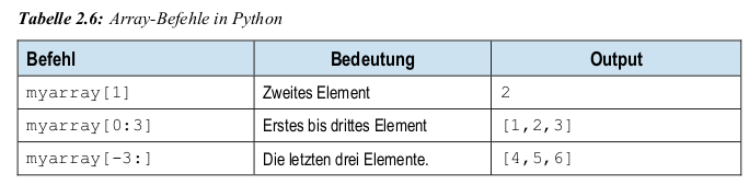
Numpy arrays und Pandas series

einzelne Elemente eines Arrays sollen zum gleichen Datentyp gehören
jedem Element eines Arrays ist eine Indexnummer zugeordnet, die den Zugriff auf das Element ermöglicht
```
import numpy as np
np.array(data)
myarray = np.array([1,2,3,4,5,6])
```

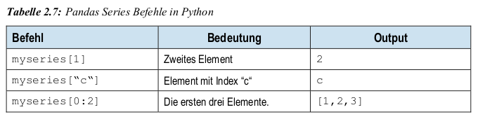
Pandas series

Pandas Series unterstützt u. a. folgende Datentypen: Ganzzahlen, Fließkommazahlen, Zeichenketten

Jedem Wert in einer Pandas Series ist ein Index zugewiesen

import pandas as pdf
myseries = pd.Series([1,2,3,4])
myseries = pd.Series([1,2,3,4], index = [“a“,“b“,“c“,“d“])

Pandas `DataFrame`

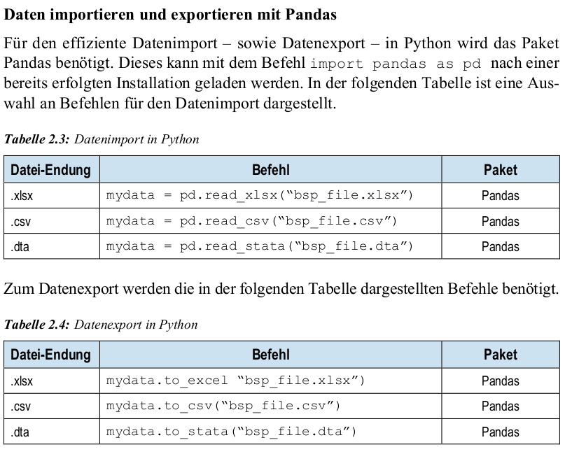
Pandas DataFrame: zweidimensionale Datenstruktur, bestehend aus n Zeilen und m Spalten und hat Zeilen- und Spaltenindizes.

mydata = {
 "Name": ["Shiva", "Tessy", "Detoterix Destroyer Of All"]
 "Dog": [1,1,0]
}
mydf = pd.DataFrame(mydata)

Graphiken:

Seaborn, Matplotlib, Plotly, Bokeh, ggplot, Altair, Geoplotlib, Gleam, Plotnine*, Pygal, und eine Menge weiterer
Das im Studienbrief SB 01, S.38-39 vorgestellte plotnine ist bewusst stark an ggplot2 angelehnt !
Pyt

R

Benötigte R-Pakete installieren