In diesem Notebook vergleichen wir verschiedene neuronale Netzarchitekturen zur Klassifikation von Bildern aus dem MNIST- und Fashion-MNIST-Datensatz.
Bibliotheken importieren
import keras as Kimport matplotlib.pyplot as pltfrom keras.models import Sequentialfrom keras.layers import Conv2D, MaxPooling2D, Flatten, Dense, Dropout
2025-08-15 16:16:55.350334: I external/local_xla/xla/tsl/cuda/cudart_stub.cc:31] Could not find cuda drivers on your machine, GPU will not be used.
2025-08-15 16:16:55.395656: I tensorflow/core/platform/cpu_feature_guard.cc:210] This TensorFlow binary is optimized to use available CPU instructions in performance-critical operations.
To enable the following instructions: AVX2 FMA, in other operations, rebuild TensorFlow with the appropriate compiler flags.
2025-08-15 16:16:56.952808: I external/local_xla/xla/tsl/cuda/cudart_stub.cc:31] Could not find cuda drivers on your machine, GPU will not be used.
MNIST-Datensatz laden und vorbereiten
Laden des Fashion-MNIST-Datensatzes aus Keras (10 Klassen, z. B. Schuhe, Pullover, Taschen)
Normalisierung der Bilddaten auf Werte im Bereich [0, 1]
Ursprünglich liegen die Grauwerte im Bereich [0, 255]
= K.datasets.mnist= mnist.load_data()= x_train / 255.0 = x_test / 255.0
Downloading data from https://storage.googleapis.com/tensorflow/tf-keras-datasets/mnist.npz
0/11490434 ━━━━━━━━━━━━━━━━━━━━ 0s 0s/step
�������������������������������������������������
9199616/11490434 ━━━━━━━━━━━━━━━━ ━━━━ 0s 0us/step
��������������������������������������������������
11490434/11490434 ━━━━━━━━━━━━━━━━━━━━ 0s 0us/step
One-Hot-Encoding der Zielvariablen
One-Hot-Encoding der Zielvariable (10 Klassen -> Vektor mit 10 Einträgen)
Beispiel: Klasse 3 -> [0, 0, 0, 1, 0, 0, 0, 0, 0, 0]
= K.utils.to_categorical(y_train)= K.utils.to_categorical(y_test)
Feedforward-Netzwerk erstellen
Ein einfaches Dense-Netz mit zwei Hidden-Layern je 128 Neuronen:
Wieder: sequentieller Aufbau eines FFNN K.models.Sequential()
Flatten-Ebene wandelt 2D-Bilder (28x28) in 1D-Vektoren (784)
zwei versteckte Dense-Schichten mit jeweils 128 Neuronen, ReLU-Aktivierung
Ausgabeschicht mit 10 Neuronen (für 10 Klassen), Softmax-Aktivierung für Wahrscheinlichkeitsverteilung
= K.models.Sequential()128 , activation= 'relu' ))128 , activation= 'relu' ))10 , activation= 'softmax' ))
Kompilieren des Modells
Adam-Optimierer
Categorical Crossentropy (für mehrklassige Klassifikation mit One-Hot-Labels)
Accuracy als Metrik
compile (= 'adam' ,= 'categorical_crossentropy' ,= ['accuracy' ]
2025-08-15 16:16:57.815219: E external/local_xla/xla/stream_executor/cuda/cuda_platform.cc:51] failed call to cuInit: INTERNAL: CUDA error: Failed call to cuInit: UNKNOWN ERROR (303)
Training des Feedforward-Netzes
30 Epochen
Batch-Größe 128
30 % der Trainingsdaten werden für Validierung verwendet
= model.fit(= 30 ,= 128 ,= 0.3 ,= 2 )
Epoch 1/30
329/329 - 2s - 6ms/step - accuracy: 0.8965 - loss: 0.3714 - val_accuracy: 0.9450 - val_loss: 0.1880
Epoch 2/30
329/329 - 1s - 3ms/step - accuracy: 0.9570 - loss: 0.1487 - val_accuracy: 0.9586 - val_loss: 0.1390
Epoch 3/30
329/329 - 1s - 3ms/step - accuracy: 0.9696 - loss: 0.1017 - val_accuracy: 0.9617 - val_loss: 0.1285
Epoch 4/30
329/329 - 1s - 3ms/step - accuracy: 0.9778 - loss: 0.0760 - val_accuracy: 0.9666 - val_loss: 0.1107
Epoch 5/30
329/329 - 1s - 3ms/step - accuracy: 0.9822 - loss: 0.0588 - val_accuracy: 0.9684 - val_loss: 0.1080
Epoch 6/30
329/329 - 1s - 3ms/step - accuracy: 0.9862 - loss: 0.0470 - val_accuracy: 0.9721 - val_loss: 0.0993
Epoch 7/30
329/329 - 1s - 3ms/step - accuracy: 0.9892 - loss: 0.0375 - val_accuracy: 0.9718 - val_loss: 0.0986
Epoch 8/30
329/329 - 1s - 3ms/step - accuracy: 0.9901 - loss: 0.0311 - val_accuracy: 0.9721 - val_loss: 0.1016
Epoch 9/30
329/329 - 1s - 3ms/step - accuracy: 0.9930 - loss: 0.0248 - val_accuracy: 0.9717 - val_loss: 0.1056
Epoch 10/30
329/329 - 1s - 3ms/step - accuracy: 0.9942 - loss: 0.0192 - val_accuracy: 0.9728 - val_loss: 0.1056
Epoch 11/30
329/329 - 1s - 3ms/step - accuracy: 0.9942 - loss: 0.0179 - val_accuracy: 0.9683 - val_loss: 0.1205
Epoch 12/30
329/329 - 1s - 3ms/step - accuracy: 0.9945 - loss: 0.0178 - val_accuracy: 0.9735 - val_loss: 0.1141
Epoch 13/30
329/329 - 1s - 3ms/step - accuracy: 0.9974 - loss: 0.0097 - val_accuracy: 0.9730 - val_loss: 0.1170
Epoch 14/30
329/329 - 1s - 3ms/step - accuracy: 0.9970 - loss: 0.0098 - val_accuracy: 0.9727 - val_loss: 0.1251
Epoch 15/30
329/329 - 1s - 3ms/step - accuracy: 0.9956 - loss: 0.0128 - val_accuracy: 0.9699 - val_loss: 0.1364
Epoch 16/30
329/329 - 1s - 3ms/step - accuracy: 0.9966 - loss: 0.0103 - val_accuracy: 0.9741 - val_loss: 0.1183
Epoch 17/30
329/329 - 1s - 3ms/step - accuracy: 0.9979 - loss: 0.0069 - val_accuracy: 0.9742 - val_loss: 0.1185
Epoch 18/30
329/329 - 1s - 3ms/step - accuracy: 0.9977 - loss: 0.0079 - val_accuracy: 0.9738 - val_loss: 0.1293
Epoch 19/30
329/329 - 1s - 3ms/step - accuracy: 0.9987 - loss: 0.0058 - val_accuracy: 0.9727 - val_loss: 0.1384
Epoch 20/30
329/329 - 1s - 3ms/step - accuracy: 0.9979 - loss: 0.0070 - val_accuracy: 0.9679 - val_loss: 0.1708
Epoch 21/30
329/329 - 1s - 3ms/step - accuracy: 0.9969 - loss: 0.0098 - val_accuracy: 0.9742 - val_loss: 0.1335
Epoch 22/30
329/329 - 1s - 3ms/step - accuracy: 0.9990 - loss: 0.0032 - val_accuracy: 0.9754 - val_loss: 0.1362
Epoch 23/30
329/329 - 1s - 3ms/step - accuracy: 0.9975 - loss: 0.0082 - val_accuracy: 0.9743 - val_loss: 0.1427
Epoch 24/30
329/329 - 1s - 3ms/step - accuracy: 0.9973 - loss: 0.0086 - val_accuracy: 0.9739 - val_loss: 0.1453
Epoch 25/30
329/329 - 1s - 3ms/step - accuracy: 0.9968 - loss: 0.0097 - val_accuracy: 0.9741 - val_loss: 0.1527
Epoch 26/30
329/329 - 1s - 3ms/step - accuracy: 0.9974 - loss: 0.0074 - val_accuracy: 0.9744 - val_loss: 0.1455
Epoch 27/30
329/329 - 1s - 3ms/step - accuracy: 0.9980 - loss: 0.0057 - val_accuracy: 0.9730 - val_loss: 0.1586
Epoch 28/30
329/329 - 1s - 3ms/step - accuracy: 0.9987 - loss: 0.0039 - val_accuracy: 0.9742 - val_loss: 0.1500
Epoch 29/30
329/329 - 1s - 3ms/step - accuracy: 0.9995 - loss: 0.0020 - val_accuracy: 0.9746 - val_loss: 0.1523
Epoch 30/30
329/329 - 1s - 3ms/step - accuracy: 0.9998 - loss: 9.3368e-04 - val_accuracy: 0.9771 - val_loss: 0.1387
Hinweise:
Das history-Objekt speichert den gesamten Trainingsverlauf (Loss und Accuracy je Epoche)
Nur dadurch ist es möglich, die Trainings- und Validierungskurven im Nachhinein zu plotten
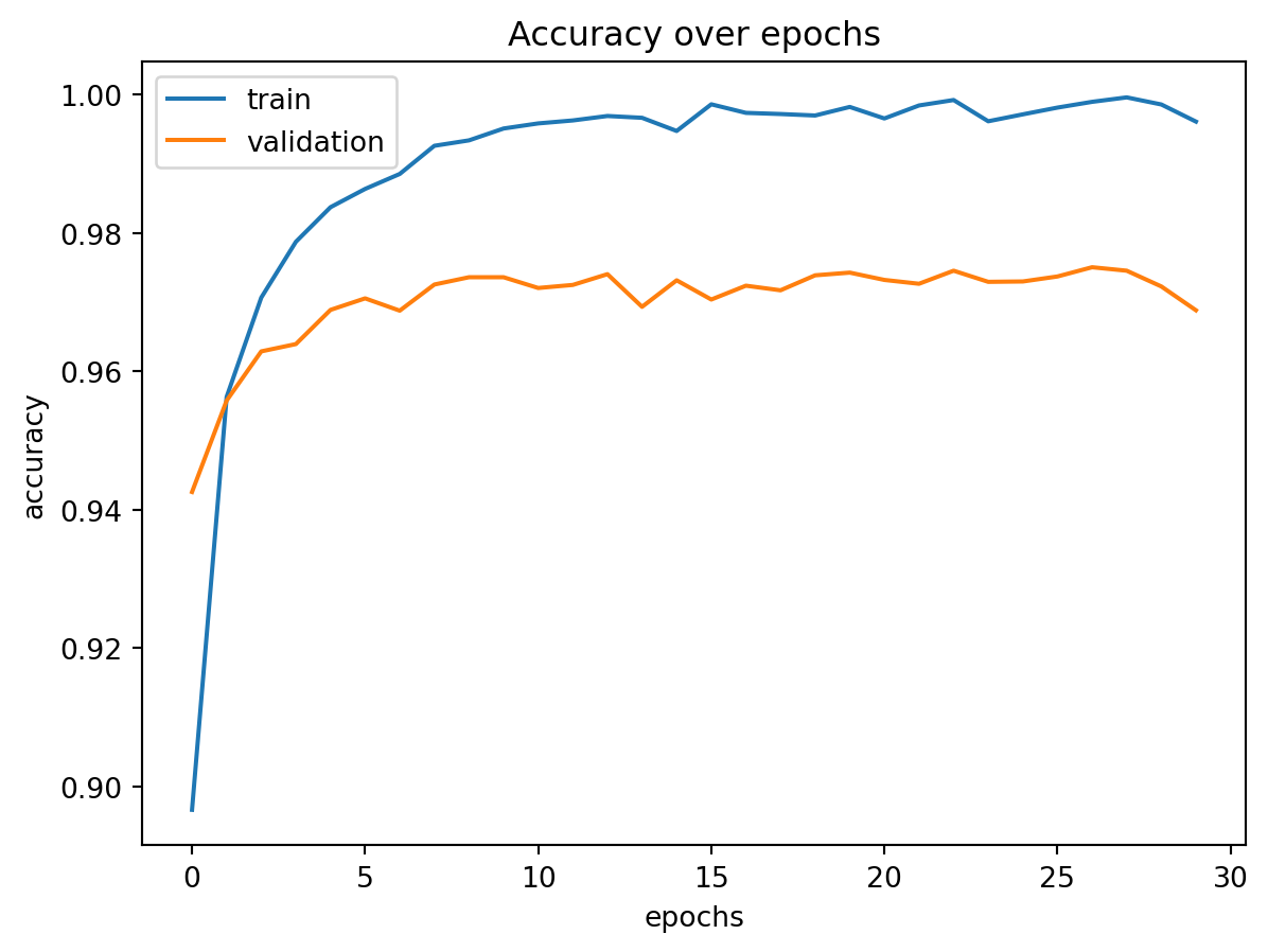
Die resultierende Grafik zeigt beide Verläufe (Accuracy auf Trainings- und Validierungsdaten)
Bei einfachem MNIST (Ziffern 0–9) erreicht das Netz bereits sehr hohe Genauigkeit
Im Vergleich dazu ist Fashion-MNIST (Kleidungsstücke) komplexer und führt zu geringerer Genauigkeit
Ursache: visuelle Ähnlichkeit mancher Klassen (z. B. Shirt vs. Pullover)
Trainingsverlauf (Feedforward-Netz)
Vergleich im Trainingsdatensatz von sowohl Train- als auch Validationsaccuracy
= plt.subplots()'Accuracy over epochs' )'epochs' )'accuracy' )'accuracy' ], label= 'train' )'val_accuracy' ], label= 'validation' )= 'upper left' )'../figs/mnist_accuracy.png' )
<Figure size 672x480 with 0 Axes>
Convolutional Neural Networks (CNN) mit Fashion-MNIST
Ziel: Verbesserung der Genauigkeit gegenüber einem einfachen Feedforward-Netz.
= K.datasets.fashion_mnist= fashion.load_data()= x_train_mf / 255.0 = x_test_mf / 255.0 = K.utils.to_categorical(y_train_mf)= K.utils.to_categorical(y_test_mf)
Downloading data from https://storage.googleapis.com/tensorflow/tf-keras-datasets/train-labels-idx1-ubyte.gz
0/29515 ━━━━━━━━━━━━━━━━━━━━ 0s 0s/step
�������������������������������������������
29515/29515 ━━━━━━━━━━━━━━━━━━━━ 0s 0us/step
Downloading data from https://storage.googleapis.com/tensorflow/tf-keras-datasets/train-images-idx3-ubyte.gz
0/26421880 ━━━━━━━━━━━━━━━━━━━━ 0s 0s/step
�������������������������������������������������
6021120/26421880 ━━━━ ━━━━━━━━━━━━━━━━ 0s 0us/step
��������������������������������������������������
13066240/26421880 ━━━━━━━━━ ━━━━━━━━━━━ 0s 0us/step
��������������������������������������������������
22061056/26421880 ━━━━━━━━━━━━━━━━ ━━━━ 0s 0us/step
��������������������������������������������������
26421880/26421880 ━━━━━━━━━━━━━━━━━━━━ 0s 0us/step
Downloading data from https://storage.googleapis.com/tensorflow/tf-keras-datasets/t10k-labels-idx1-ubyte.gz
0/5148 ━━━━━━━━━━━━━━━━━━━━ 0s 0s/step
�����������������������������������������
5148/5148 ━━━━━━━━━━━━━━━━━━━━ 0s 0us/step
Downloading data from https://storage.googleapis.com/tensorflow/tf-keras-datasets/t10k-images-idx3-ubyte.gz
0/4422102 ━━━━━━━━━━━━━━━━━━━━ 0s 0s/step
�����������������������������������������������
4422102/4422102 ━━━━━━━━━━━━━━━━━━━━ 0s 0us/step
CNN-Architektur definieren
Der erste Layer ist ein Conv2D-Layer:
32 Filter mit einer Kerneldimension von 3×3ReLU -Aktivierunginput_shape=(28, 28, 1): Eingabebilder sind 28×28 Pixel mit 1 Kanal (grau) Anschließend reduziert ein **MaxPooling2D-Layer* die räumliche Dimension der Featuremaps
Der Flatten-Layer wandelt die 2D-Ausgabe in einen 1D-Vektor um, sodass dieser an vollverbundene (Dense) Schichten übergeben werden kann
Eine Dense-Schicht mit 100 Neuronen und **ReLU-Aktivierung* als Hidden-Layer
Ausgabeschicht für 10 Klassen (z. B. Ziffern oder Kleidungsstücke), Softmax-Aktivierung liefert Wahrscheinlichkeiten
= Sequential()32 , (3 , 3 ), activation = 'relu' , input_shape= (28 , 28 , 1 )))2 , 2 )))100 , activation = 'relu' ))10 , activation = 'softmax' ))
/opt/hostedtoolcache/Python/3.10.18/x64/lib/python3.10/site-packages/keras/src/layers/convolutional/base_conv.py:113: UserWarning:

Do not pass an `input_shape`/`input_dim` argument to a layer. When using Sequential models, prefer using an `Input(shape)` object as the first layer in the model instead.
Kompilierung des CNN-Modells
Optimierer: Adam (effizient, adaptiv)
Verlustfunktion: categorical_crossentropy (geeignet für mehrklassige Klassifikation mit One-Hot-Labels)
Metrik: accuracy
compile (= 'adam' , loss = 'categorical_crossentropy' ,= ['accuracy' ])
= x_train_mf.reshape(- 1 , 28 , 28 , 1 )= x_test_mf.reshape(- 1 , 28 , 28 , 1 )
Training des CNNs auf Fashion-MNIST
x_train_mf und y_train_mf: normalisierte Trainingsbilder und One-Hot-Labelsx_test_mf und y_test_mf: Testdaten zur Validierung30 Epochen, Batch-Größe 128
= model2.fit(= 30 ,= 128 ,= (x_test_mf, y_test_mf),= 2
Epoch 1/30
469/469 - 9s - 19ms/step - accuracy: 0.8462 - loss: 0.4441 - val_accuracy: 0.8760 - val_loss: 0.3517
Epoch 2/30
469/469 - 7s - 16ms/step - accuracy: 0.8953 - loss: 0.2953 - val_accuracy: 0.8881 - val_loss: 0.3020
Epoch 3/30
469/469 - 7s - 15ms/step - accuracy: 0.9079 - loss: 0.2564 - val_accuracy: 0.9003 - val_loss: 0.2770
Epoch 4/30
469/469 - 7s - 16ms/step - accuracy: 0.9186 - loss: 0.2265 - val_accuracy: 0.9004 - val_loss: 0.2690
Epoch 5/30
469/469 - 7s - 15ms/step - accuracy: 0.9237 - loss: 0.2076 - val_accuracy: 0.9080 - val_loss: 0.2578
Epoch 6/30
469/469 - 7s - 15ms/step - accuracy: 0.9309 - loss: 0.1904 - val_accuracy: 0.9109 - val_loss: 0.2493
Epoch 7/30
469/469 - 7s - 15ms/step - accuracy: 0.9375 - loss: 0.1710 - val_accuracy: 0.9089 - val_loss: 0.2554
Epoch 8/30
469/469 - 7s - 16ms/step - accuracy: 0.9427 - loss: 0.1570 - val_accuracy: 0.9153 - val_loss: 0.2502
Epoch 9/30
469/469 - 7s - 16ms/step - accuracy: 0.9483 - loss: 0.1448 - val_accuracy: 0.9162 - val_loss: 0.2426
Epoch 10/30
469/469 - 10s - 22ms/step - accuracy: 0.9513 - loss: 0.1345 - val_accuracy: 0.9172 - val_loss: 0.2451
Epoch 11/30
469/469 - 7s - 15ms/step - accuracy: 0.9572 - loss: 0.1190 - val_accuracy: 0.9151 - val_loss: 0.2610
Epoch 12/30
469/469 - 7s - 15ms/step - accuracy: 0.9598 - loss: 0.1099 - val_accuracy: 0.9190 - val_loss: 0.2612
Epoch 13/30
469/469 - 7s - 15ms/step - accuracy: 0.9627 - loss: 0.1021 - val_accuracy: 0.9146 - val_loss: 0.2725
Epoch 14/30
469/469 - 7s - 15ms/step - accuracy: 0.9676 - loss: 0.0913 - val_accuracy: 0.9149 - val_loss: 0.2916
Epoch 15/30
469/469 - 7s - 15ms/step - accuracy: 0.9702 - loss: 0.0824 - val_accuracy: 0.9183 - val_loss: 0.2832
Epoch 16/30
469/469 - 7s - 16ms/step - accuracy: 0.9747 - loss: 0.0732 - val_accuracy: 0.9129 - val_loss: 0.3137
Epoch 17/30
469/469 - 7s - 15ms/step - accuracy: 0.9772 - loss: 0.0658 - val_accuracy: 0.9181 - val_loss: 0.3001
Epoch 18/30
469/469 - 7s - 15ms/step - accuracy: 0.9783 - loss: 0.0622 - val_accuracy: 0.9117 - val_loss: 0.3264
Epoch 19/30
469/469 - 7s - 16ms/step - accuracy: 0.9819 - loss: 0.0533 - val_accuracy: 0.9190 - val_loss: 0.3113
Epoch 20/30
469/469 - 7s - 15ms/step - accuracy: 0.9827 - loss: 0.0499 - val_accuracy: 0.9135 - val_loss: 0.3659
Epoch 21/30
469/469 - 7s - 15ms/step - accuracy: 0.9857 - loss: 0.0425 - val_accuracy: 0.9157 - val_loss: 0.3499
Epoch 22/30
469/469 - 7s - 15ms/step - accuracy: 0.9877 - loss: 0.0376 - val_accuracy: 0.9160 - val_loss: 0.3729
Epoch 23/30
469/469 - 7s - 16ms/step - accuracy: 0.9885 - loss: 0.0344 - val_accuracy: 0.9162 - val_loss: 0.3772
Epoch 24/30
469/469 - 7s - 15ms/step - accuracy: 0.9895 - loss: 0.0320 - val_accuracy: 0.9122 - val_loss: 0.4280
Epoch 25/30
469/469 - 7s - 15ms/step - accuracy: 0.9888 - loss: 0.0321 - val_accuracy: 0.9140 - val_loss: 0.4163
Epoch 26/30
469/469 - 7s - 16ms/step - accuracy: 0.9917 - loss: 0.0250 - val_accuracy: 0.9152 - val_loss: 0.4080
Epoch 27/30
469/469 - 7s - 16ms/step - accuracy: 0.9911 - loss: 0.0269 - val_accuracy: 0.9176 - val_loss: 0.4133
Epoch 28/30
469/469 - 7s - 16ms/step - accuracy: 0.9932 - loss: 0.0229 - val_accuracy: 0.9136 - val_loss: 0.4390
Epoch 29/30
469/469 - 7s - 16ms/step - accuracy: 0.9934 - loss: 0.0203 - val_accuracy: 0.9144 - val_loss: 0.4733
Epoch 30/30
469/469 - 7s - 16ms/step - accuracy: 0.9954 - loss: 0.0165 - val_accuracy: 0.9175 - val_loss: 0.4419
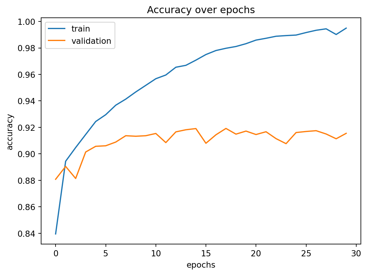
Visualisierung des CNN-Trainingsverlaufs
= plt.subplots()'Accuracy over epochs' )'epochs' )'accuracy' )'accuracy' ], label = 'train' )'val_accuracy' ], label = 'validation' )= 'upper left' )'../figs/mnist_accuracy_convolutional.png' )
<Figure size 672x480 with 0 Axes>
Zusammenfassung
Das CNN beginnt mit einem Conv2D-Layer:
Er verwendet 32 Filter mit einer Kernelgröße von 3x3
Diese extrahieren lokale Bildmerkmale (z. B. Kanten, Texturen)
Die erste Zahl (32) gibt die Anzahl der Filter (= Ausgabekanäle) an
Eine höhere Anzahl an Filtern erhöht die Modellkapazität, aber auch den Rechenaufwand
In empirischen Tests zeigt sich: - Bereits einfache CNNs erreichen ~99 % Trainingsgenauigkeit und ~91 % Testgenauigkeit - Dies entspricht einem signifikanten Fortschritt gegenüber klassischen Feedforward-Netzen
Für eine bessere Generalisierbarkeit wurden zusätzliche Experimente durchgeführt: - Variation der Anzahl der Filter im ersten Conv2D-Layer (z. B. 32, 40, 48, 56) - Das Modell mit 48 Filtern schnitt im Mittel am besten auf den Testdaten ab
Eine weitere bewährte Technik zur Vermeidung von Overfitting ist der Einsatz eines Dropout-Layers: - Während des Trainings werden zufällig ausgewählte Neuronen deaktiviert - Dies verhindert eine zu starke Abhängigkeit von einzelnen Aktivierungen - Ziel: bessere Generalisierbarkeit auf unbekannte Daten
CNN mit Dropout zur Vermeidung von Overfitting
Ein Dropout-Layer deaktiviert während des Trainings zufällig 10 % der Neuronen im vorherigen Layer. Ziel: Netz soll robuster gegen Überanpassung werden und besser auf neuen Daten generalisieren
= Sequential()32 , (3 , 3 ), activation = 'relu' , input_shape= (28 , 28 , 1 )))2 , 2 )))0.1 )) # 10 % der Neuronen werden zufällig deaktiviert 100 , activation = 'relu' ))10 , activation = 'softmax' ))