In diesem Notebook führen wir die vollständige Datenaufbereitung, Modellierung, Visualisierung und Evaluierung eines neuronalen Netzes zur Unterscheidung von Rot- und Weißwein durch.
import pandas as pdimport numpy as npimport keras as Kimport matplotlib.pyplot as pltfrom sklearn.model_selection import train_test_splitfrom sklearn.preprocessing import StandardScaler
2025-08-15 16:16:39.062033: I external/local_xla/xla/tsl/cuda/cudart_stub.cc:31] Could not find cuda drivers on your machine, GPU will not be used.
2025-08-15 16:16:39.106647: I tensorflow/core/platform/cpu_feature_guard.cc:210] This TensorFlow binary is optimized to use available CPU instructions in performance-critical operations.
To enable the following instructions: AVX2 FMA, in other operations, rebuild TensorFlow with the appropriate compiler flags.
2025-08-15 16:16:41.176874: I external/local_xla/xla/tsl/cuda/cudart_stub.cc:31] Could not find cuda drivers on your machine, GPU will not be used.
Einlesen der Weindaten
Die CSV-Dateien befinden sich im Unterordner data/processed. Sie enthalten standardisierte chemische Merkmale für Rot- und Weißweine.
white = pd.read_csv('../data/processed/winequality-white.csv', sep=';')red = pd.read_csv('../data/processed/winequality-red.csv', sep=';')
Labeln und Zusammenführen der Datensätze
Für supervised learning bönitgen wir labels: - Rotwein erhält das Label 1 - Weißwein das Label 0
Die ersten 11 Spalten (chemische Eigenschaften) dienen als Input-Variablen (Features). Die Zielvariable y ist das binäre Label (1 = Rotwein, 0 = Weißwein), und wird in 1D-Array umgewandelt.
x = wines.iloc[:, 0:11]y = np.ravel(wines['label'])
Aufteilung in Trainings- und Testdaten
Der Datensatz wird im Verhältnis 70:30 in Trainings- und Testdaten aufgeteilt (70% Trainingsdaten).
Die Daten werden mit dem StandardScaler auf Mittelwert 0 und Standardabweichung 1 standardisiert. Unterschiedliche Skalen der Inputvariablen (z. B. pH vs. Alkohol) können das Training stören. Der Fit erfolgt nur auf dem Trainingsset, aber: Testdaten müssen auch transformiert werden.
Das neuronale Netz wird an diese Problemstruktur angepasst: - ein einzelnes Ausgabeneuron mit Sigmoid-Aktivierung (für binäre Klassifikation) - Eingabedimension entspricht der Anzahl der Input-Features (hier: 11)
Aufbau des neuronalen Netzes
Wir definieren ein sequentielles Keras-Modell, , in dem Layer nacheinander hinzugefügt werden. Hyperparameter wie Anzahl der Hidden-Layer, Neuronenanzahl, Aktivierungsfunktionen etc. sind frei wählbar. Die Sturktur ist wie folgt: - Eingabeschicht: 12 Neuronen, ReLU, input_dim=11 - Hidden Layer: 8 Neuronen, ReLU - Ausgabeschicht: 1 Neuron, Sigmoid (für binäre Klassifikation)
import keras as K # oder: from tensorflow import keras as Kmodel = K.Sequential([ K.layers.Input(shape=(11,)), # <<— Input-Layer K.layers.Dense(12, activation='relu'), K.layers.Dense(8, activation='relu'), K.layers.Dense(1, activation='sigmoid')])# So wurde es SB 03 gemacht, aber veraltet ...# model = K.models.Sequential()# model.add(K.layers.Dense(units=12, activation='relu', input_dim=11))# model.add(K.layers.Dense(units=8, activation='relu'))# model.add(K.layers.Dense(units=1, activation='sigmoid'))
2025-08-15 16:16:41.820203: E external/local_xla/xla/stream_executor/cuda/cuda_platform.cc:51] failed call to cuInit: INTERNAL: CUDA error: Failed call to cuInit: UNKNOWN ERROR (303)
Weitere Hintergründe
Erstellen eines sequenziellen Keras-Modells
Erste Schicht (Input-Layer + erste Dense-Schicht)
12 Neuronen als Startwert (guter Richtwert, entspricht etwa der Feature-Anzahl)
Aktivierungsfunktion: ReLU (Standard bei Hidden-Layern)
input_dim: 11, da 11 Input-Features (chemische Eigenschaften)
Zweite Schicht (Hidden-Layer)
8 Neuronen (leichte Reduktion gegenüber erster Schicht)
erneut ReLU-Aktivierung
Ausgabeschicht für binäre Klassifikation
1 Neuron (0 = rot, 1 = weiß)
Aktivierungsfunktion: Sigmoid (liefert Werte zwischen 0 und 1 geeignet für binäre Klassen)
Für mehrklassige Klassifikation würde man stattdessen:
mehrere Ausgabeneuronen (entsprechend der Klassenzahl)
und eine ‘softmax’-Aktivierung verwenden
Kompilierung des Modells
Festlegen von Optimierer, Verlustfunktion und Metriken
Optimierer: Adam (state-of-the-art für viele Probleme, adaptiv)
Verlustfunktion: binary_crossentropy (geeignet für binäre Klassifikation)
Metrik: accuracy (Anteil korrekt klassifizierter Beispiele pro Epoche)
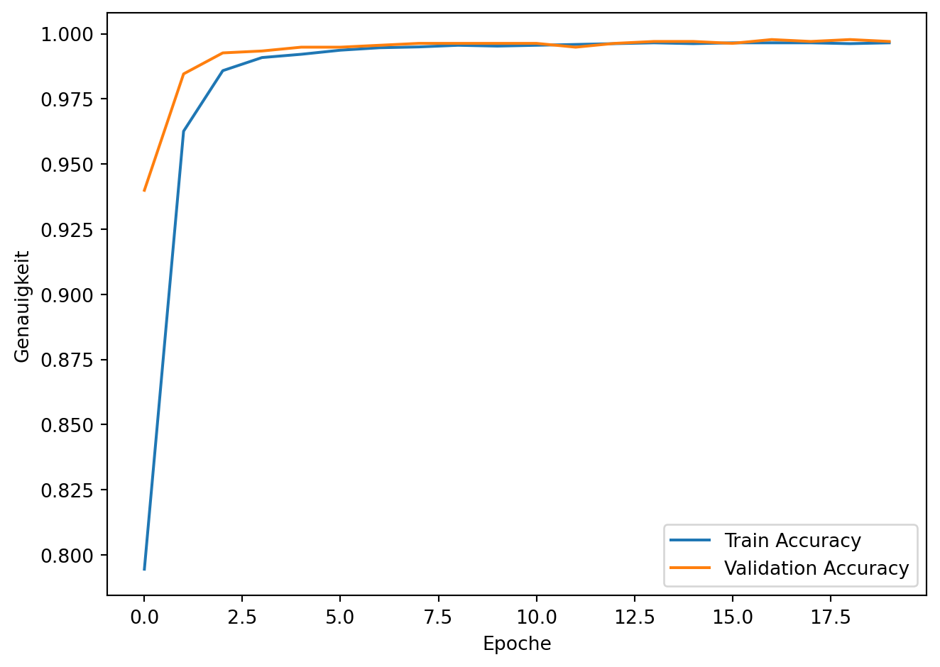
Hinweis: - Die Validierung während des Trainings basiert auf validation_split - Die finale Testgenauigkeit stammt aus einer separaten, vorher unberührten Testmenge - Dadurch erhalten wir eine realistische Einschätzung der Generalisierungsfähigkeit